Laser Cutting the Lake
A year ago, I laser-cut paper mountains, as an exploration of oblique-perspective topography, digital elevation models (DEMs), and the resources of the University’s “Hack Arts Labs” (HAL). That project got me excited about laser cutting, but just as I was getting ramped up, the world shut down. Over the past year, I thought a lot about expressing water and waves, and imagining projects that I could not satisfactorily execute with an x-acto knife.
I finally got back into HAL for few hours and made a classic laser cutting project: a bathymetric map. There are so many wood-cut maps on Etsy that it’s not even worth comparing, but I was pleased with my result. What distinguished my map is that, since I couldn’t cut anything for many months, I spent that time imagining what I would cut if I could cut, and thus whiled many hours of quarantimes painting things blue. We all need a respites from covid, and this was mine:
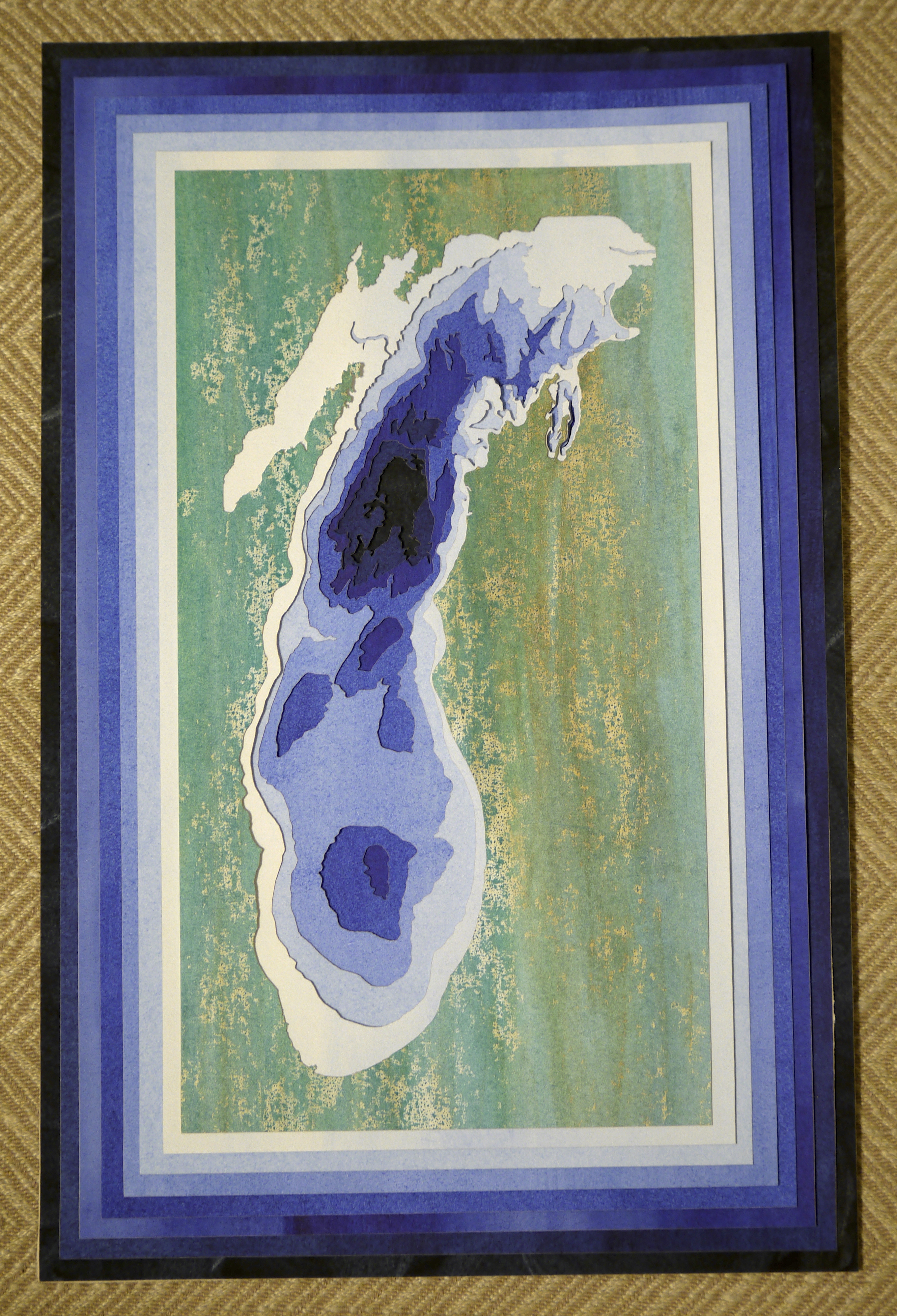
Lake Michigan bathymetry, laser cut from painted paper. (Click to expand.)
This post presents a short script for making the vector files of the bathymetry, along with my explorations of the color blue.
The Bathymetry.
As you can see from the picture above, the map consists of eight shapes, showing the shape of Lake Michigan in depth intervales of 50 meters, ranging from its surface down to 281 meters. To make this, you can start with the raster “bathymetry” (depth measurement) data of the Lake, which you can retrieve from NOAA. I used the GeoTIFF files.
The data file is just a grid with a depth measurement at each point, from which we must extract isobaths – lines connecting equal depths. (In other words, it is the same as an isocontour in a more-familiar topographic map.) Before doing this, you should convert the the data to an appropriate coordinate reference system. I use the one for Central Michigan, EPSG:3587:
gdalwarp -t_srs EPSG:3587 michigan_lld/michigan_lld.tif lake_michigan.tiff
You can get isobaths/contours from either GDAL or within python.
For gdal,
gdal_contour lake_michigan.tiff -i 50 -a elev contours.shp
Since GDAL 2.4, you can also ostensibly use the polygon option, -p (with -amin and -amax):
gdal_contour lake_michigan.tiff -i 50 -amin -500 -amax 0 -p polgyons.shp
This connects all of the appropriate lines into cuts – which up in particular at the west and north, where the Lake reaches a bit beyond the bounds of the data. Unfortunately, this takes ages (i.e., not clear if it ever actually returns).
For python, I found it easiest with scikit image. First some imports:
import matplotlib.pyplot as plt

import numpy as np
from skimage import measure

import rasterio
import geopandas as gpd
from shapely.geometry import Polygon, MultiPolygon
Then read in the data.
with rasterio.open('lake_michigan.tiff') as ds:
    arr = ds.read(1) # Specify band 1 explicitly.
I then dealt with the values outside of the projection, so that it doesn’t interfere with the contours.
arr[(arr > 0) | (arr < -1000)] = 1
Alternatively, one could mask these: np.ma.masked_where(arr == 1, arr).
Next, decide how many levels to cut, and the depth of the Lake.
Note that there is one more level to the bathymetry, than what is cut,
since there’s one under the last cut.
LAKE_DEPTH, LEVELS = 281, 7
Finally, and this is the fun part, create the contours, and create a GeoDataFrame.
polygons, polygon_depths = [], []
for v in np.arange(0, -LAKE_DEPTH, -LAKE_DEPTH/LEVELS).round():

    for c in measure.find_contours(arr.T, v):
        polygons.append(Polygon(c))
        polygon_depths.append(v)

# Convert lists to GDF.
poly_gdf = gpd.GeoDataFrame(data = {"depth" : polygon_depths},
                            geometry = polygons)
For “artistic” and practical (laser cutting) purposes, the contours that we get from this are too intricate: the “shores” of Lake Michigan wind up the banks of its tributaries, and those shores can look “pocked.” To deal with this, I remove small features (by length or area) and simplify the geometries slightly.
poly_gdf = poly_gdf[(poly_gdf.length > 250) & (poly_gdf.area > 5e3)].copy()
poly_gdf.set_geometry(poly_gdf.simplify(2), inplace = True)
poly_gdf = poly_gdf.dissolve("depth").reset_index()
In the last step, I dissolved Polygons into MultiPolygons, to make them a little easier to group and visualize. We can then just plot this and save it as an SVG to work with in Illustrator and send to the laser, one “print” per layer. Plotting the raster and vectorized data side by side, looks like this.
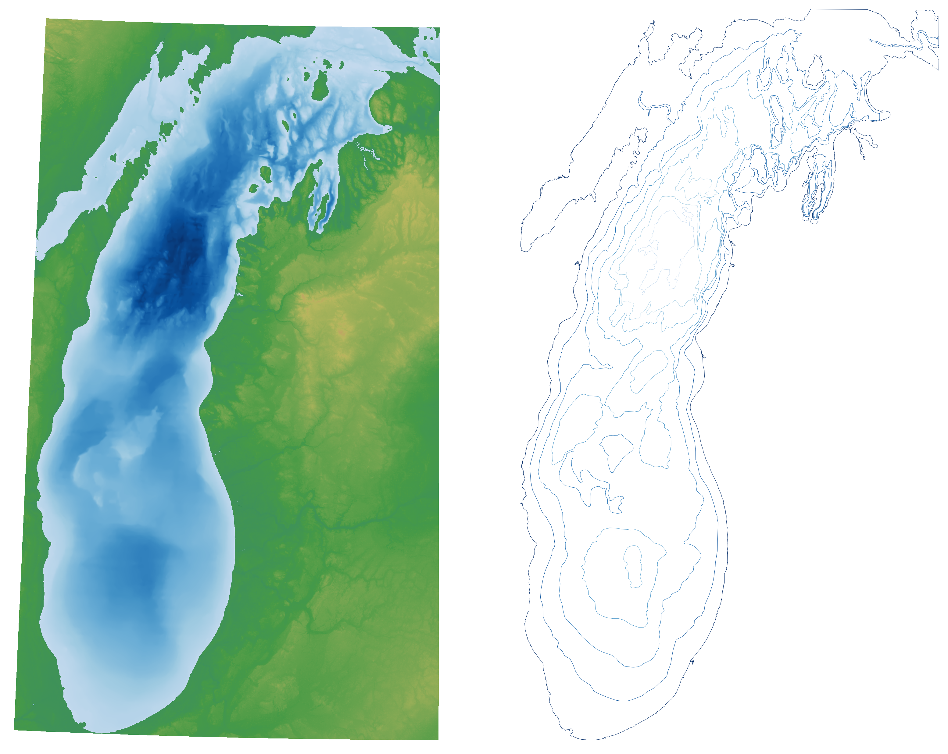
At this point, I did manipulate the files with Illustrator to remove a few streams, and the area beyond the Mackinac Straits in Lake Huron, and set the appropriate colors and linewidths for laser cutting.1
The Coloring.
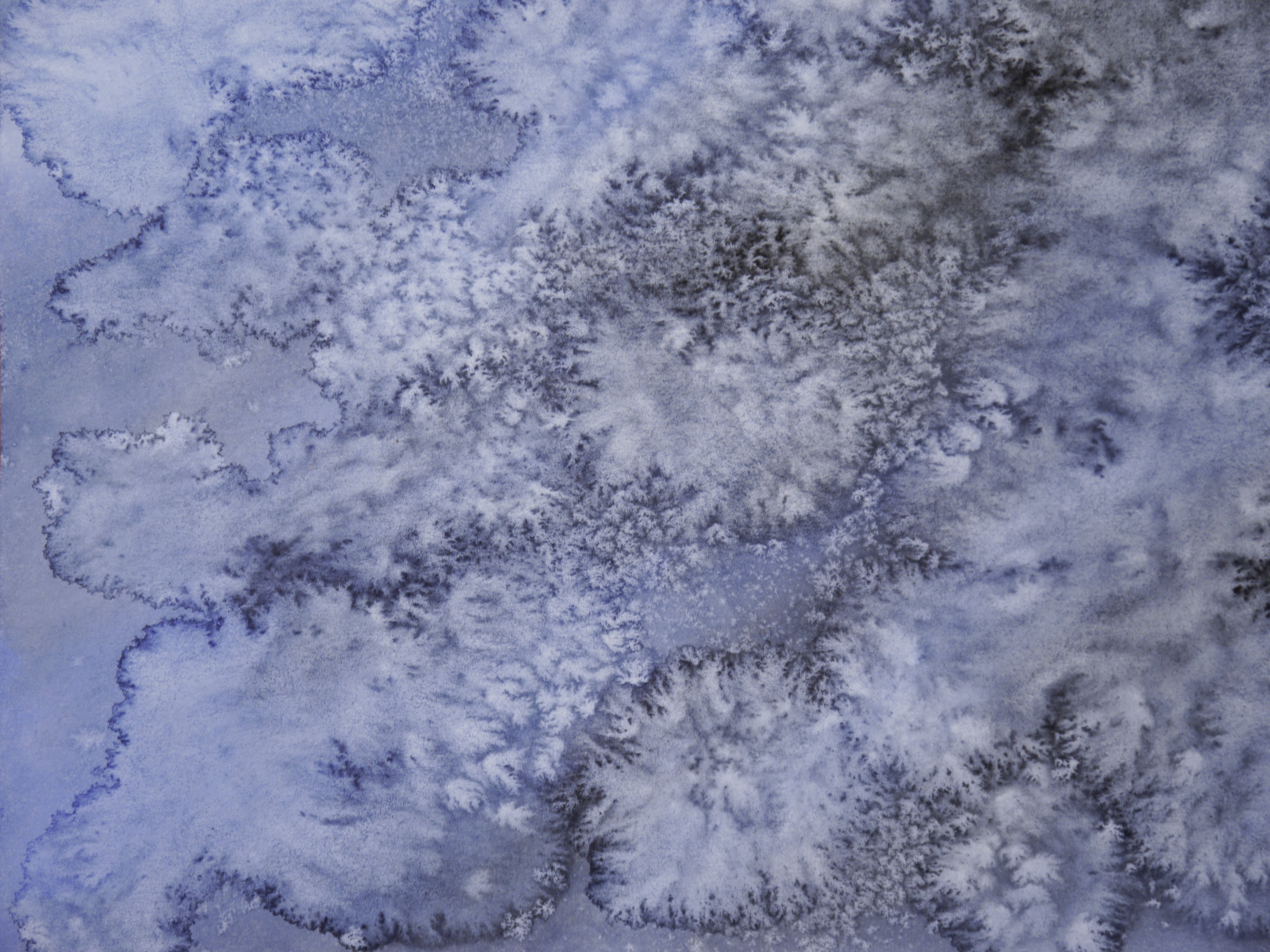
I wanted the cutting to evoke water, and so I got a bit obsessed with the color blue. I tried a lot of strategies for making things blue, but watercolors were best first and last. At first, I planned each individual sheet as a distinct technique/composition. This plan was definitely misguided: it was too busy, and it became impossible to achieve harmony in the full work.
Notwithstanding, some of this “misfire” was appealing. This was my first outing since childhood with watercolors, and I learned a good deal from a book by my sister’s friend, Sasha Prood. I also drew from the many videos of craftsy watercolor techniques on YouTube.
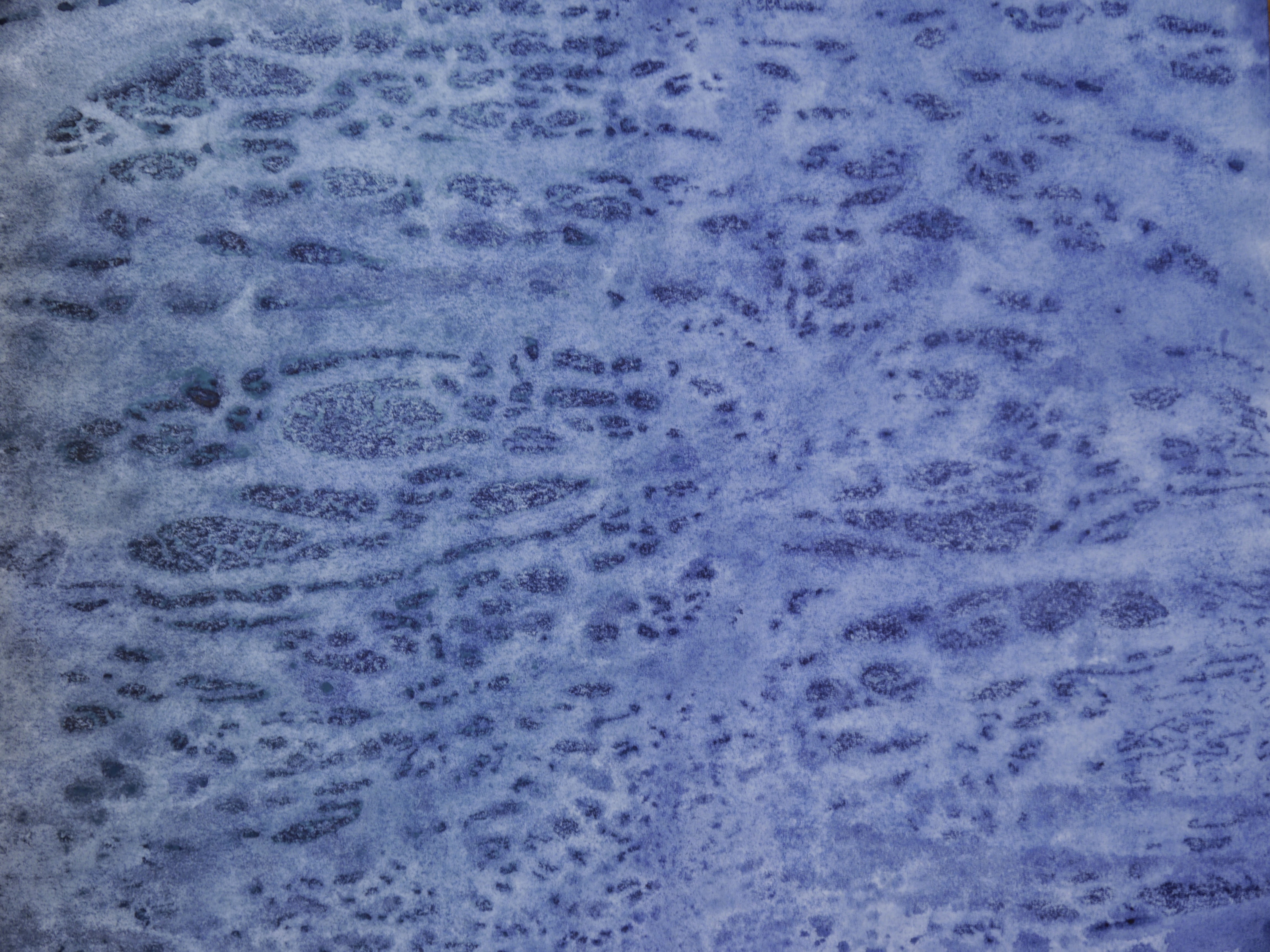
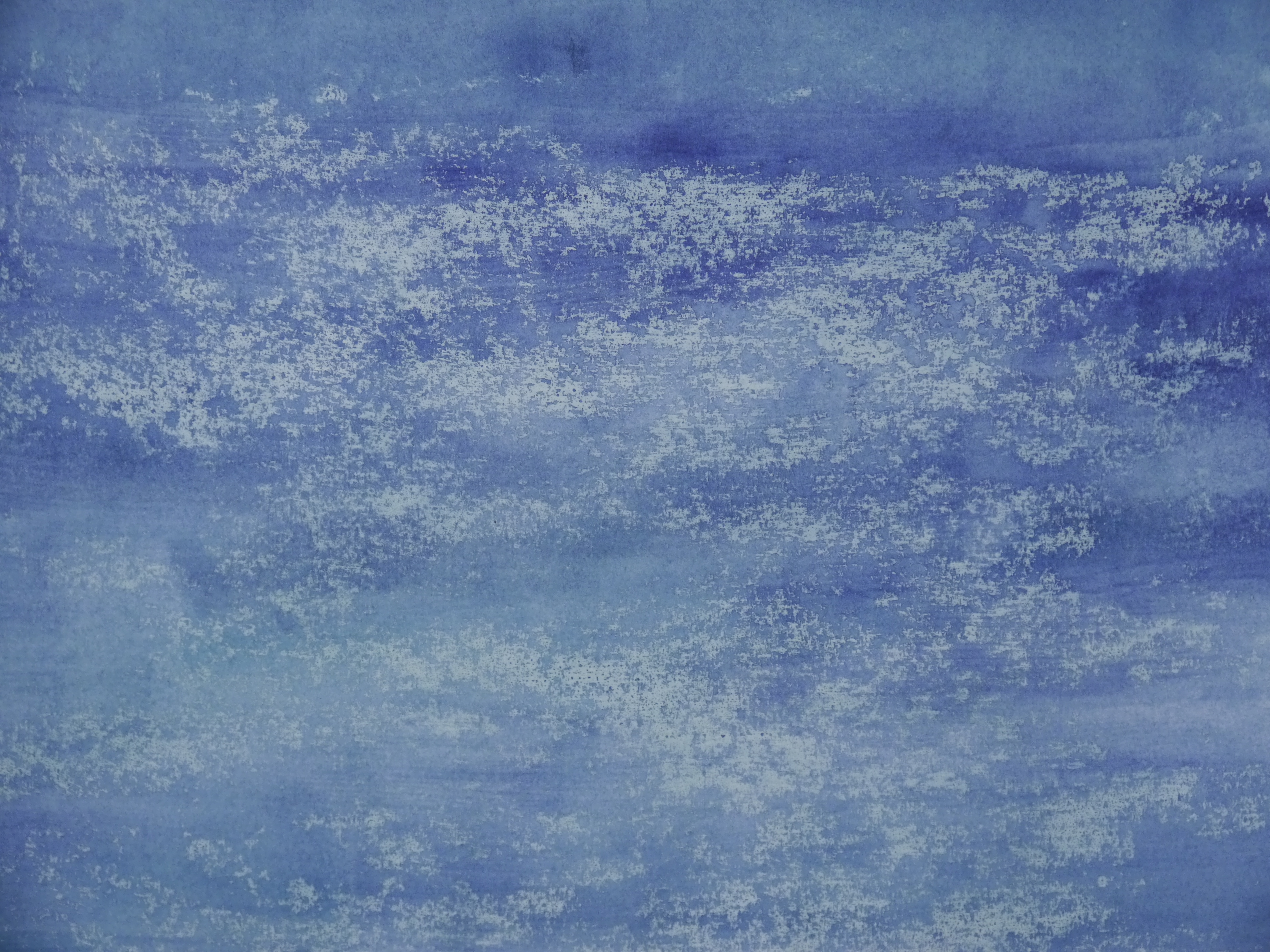
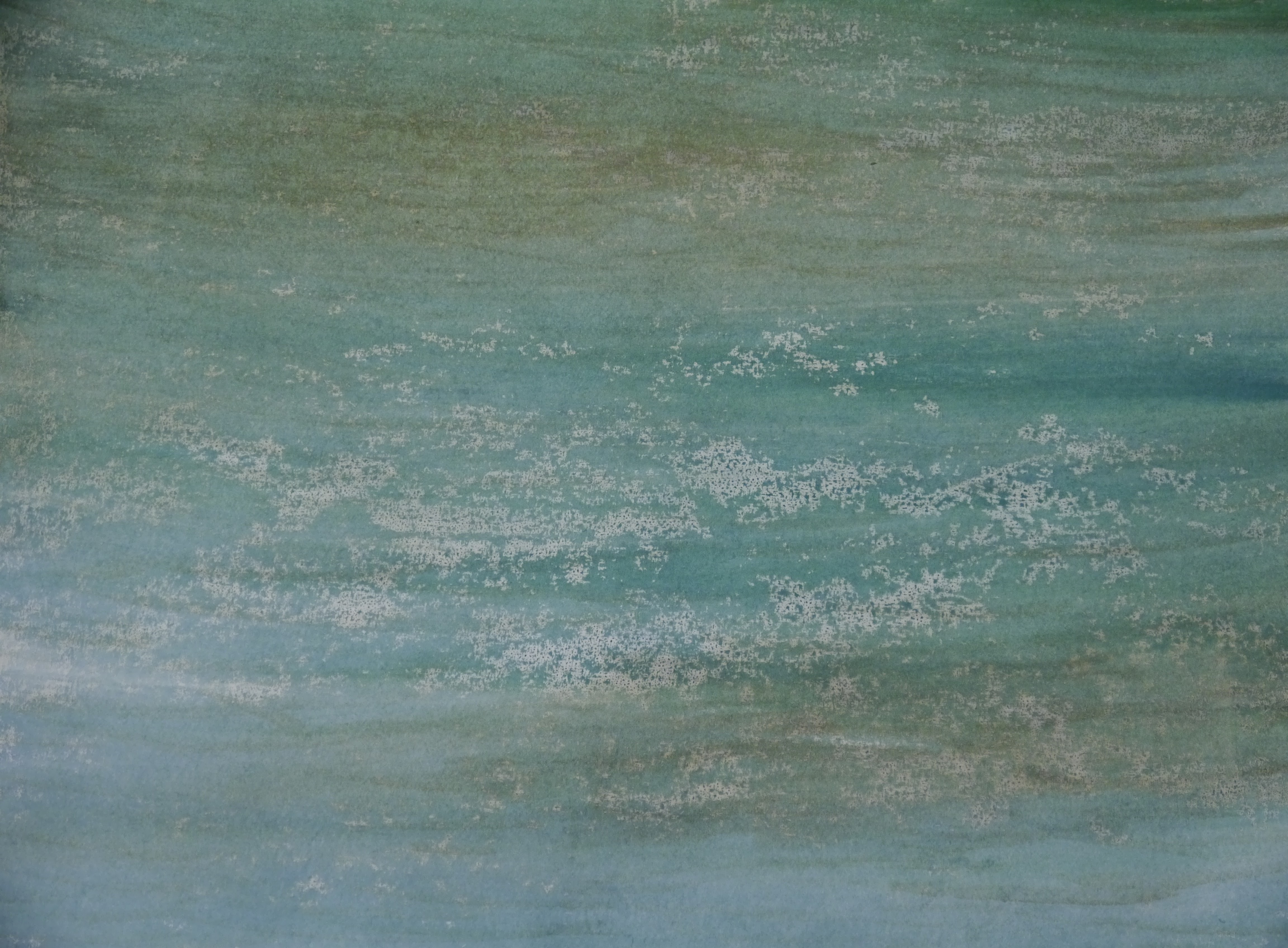
I liked the “bloom” effect created by dropping water with a syringe, but my favorite was to use parchment paper over a complete, yet still tacky piece. When this dries and the parchment paper is removed, it lifts away pigment wherever the parchment stuck to the piece. I also iterated with a “batik” process – lay down a light color, then do a wax rubbing of various natural textures with a white or light crayon, and then painting a second color. I used this single technique on the uppermost layer.
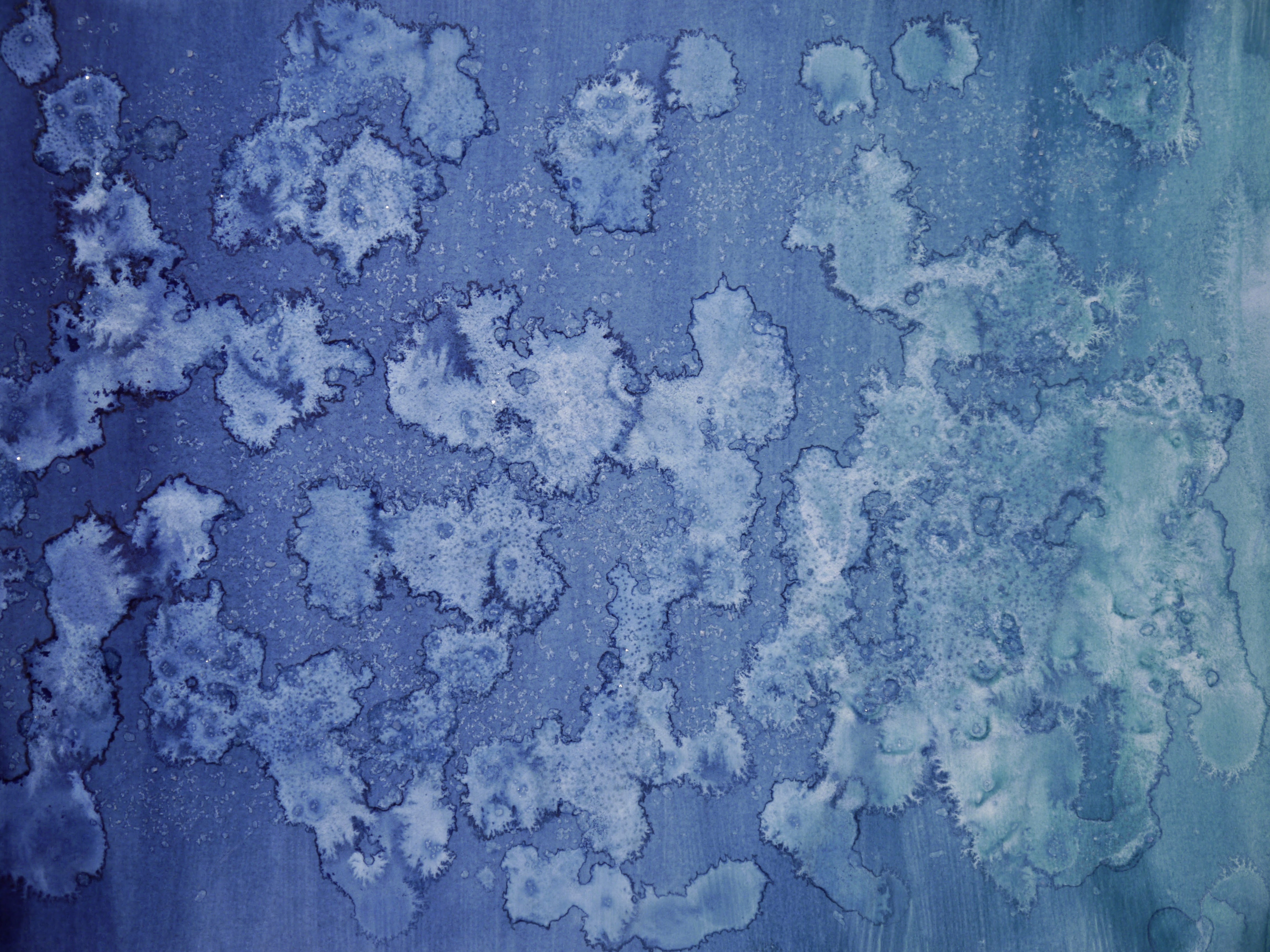
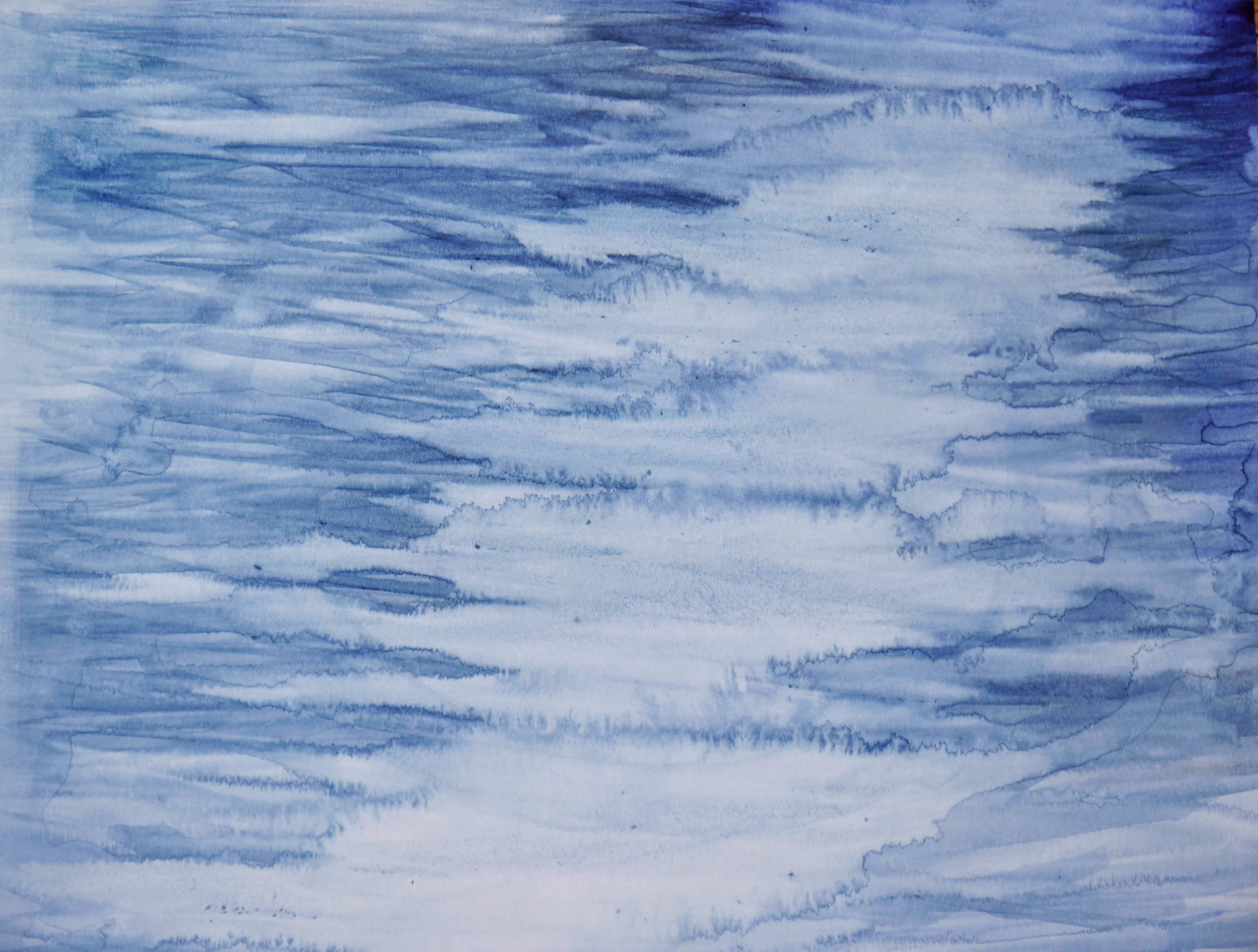
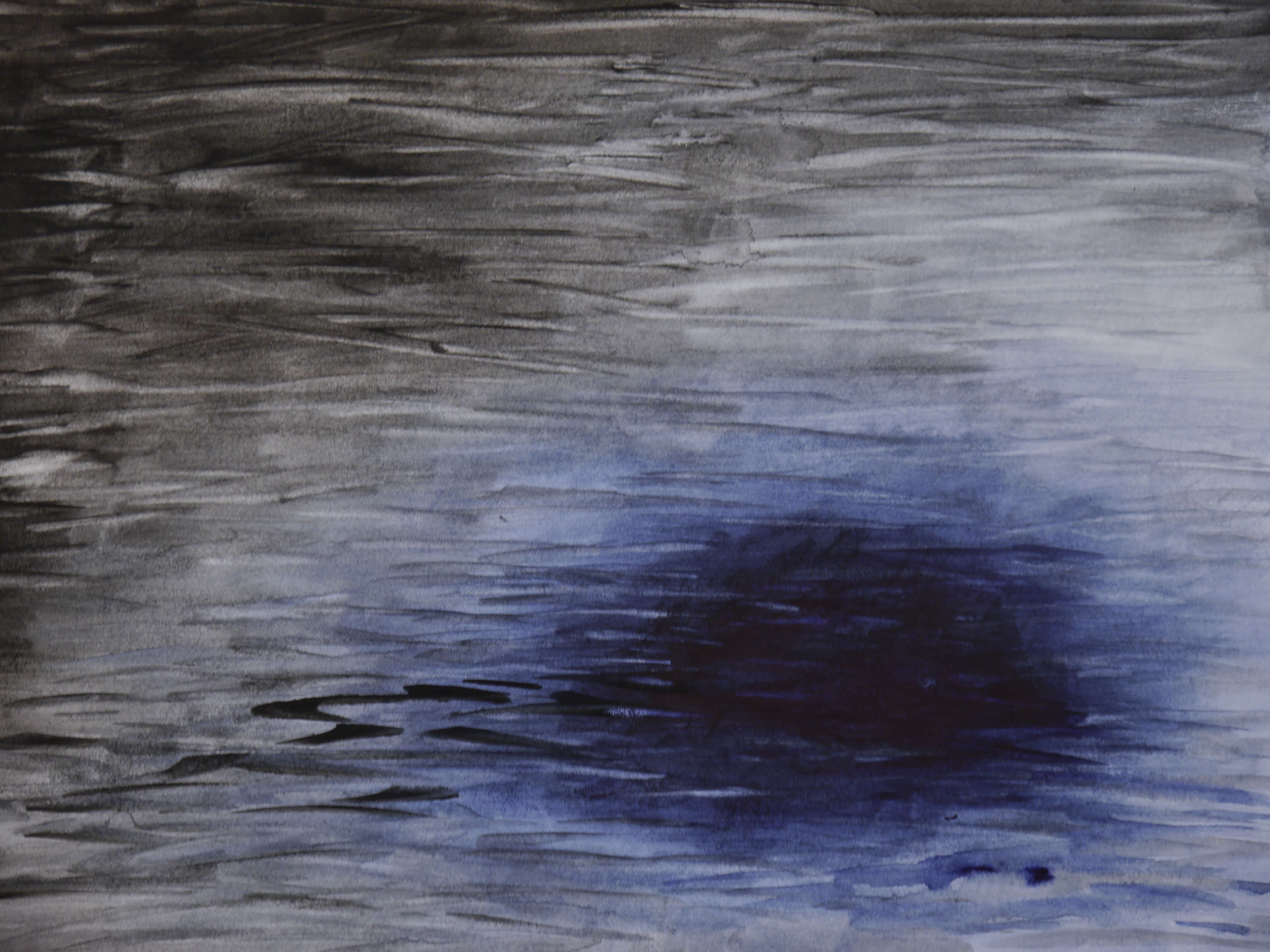
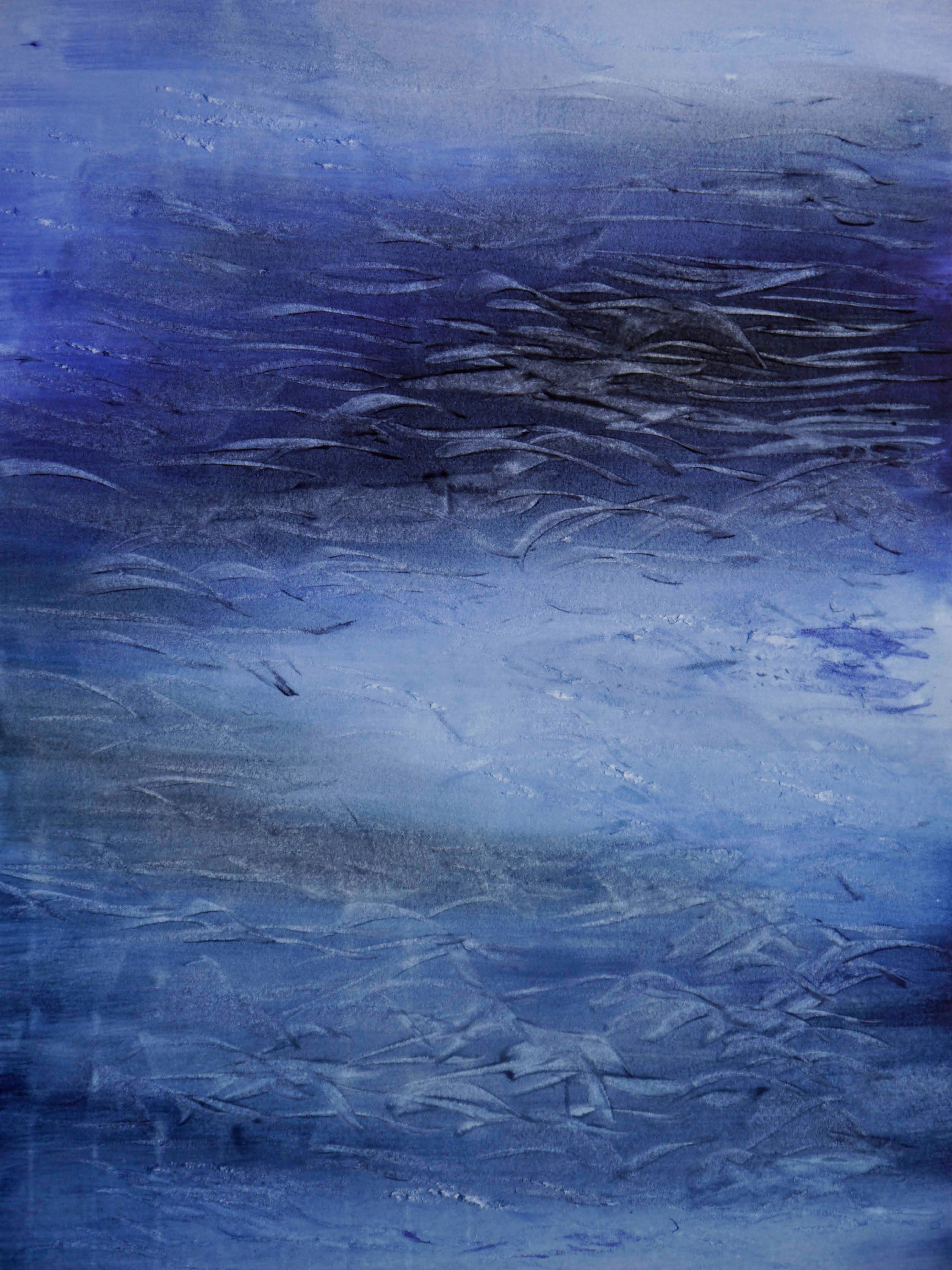
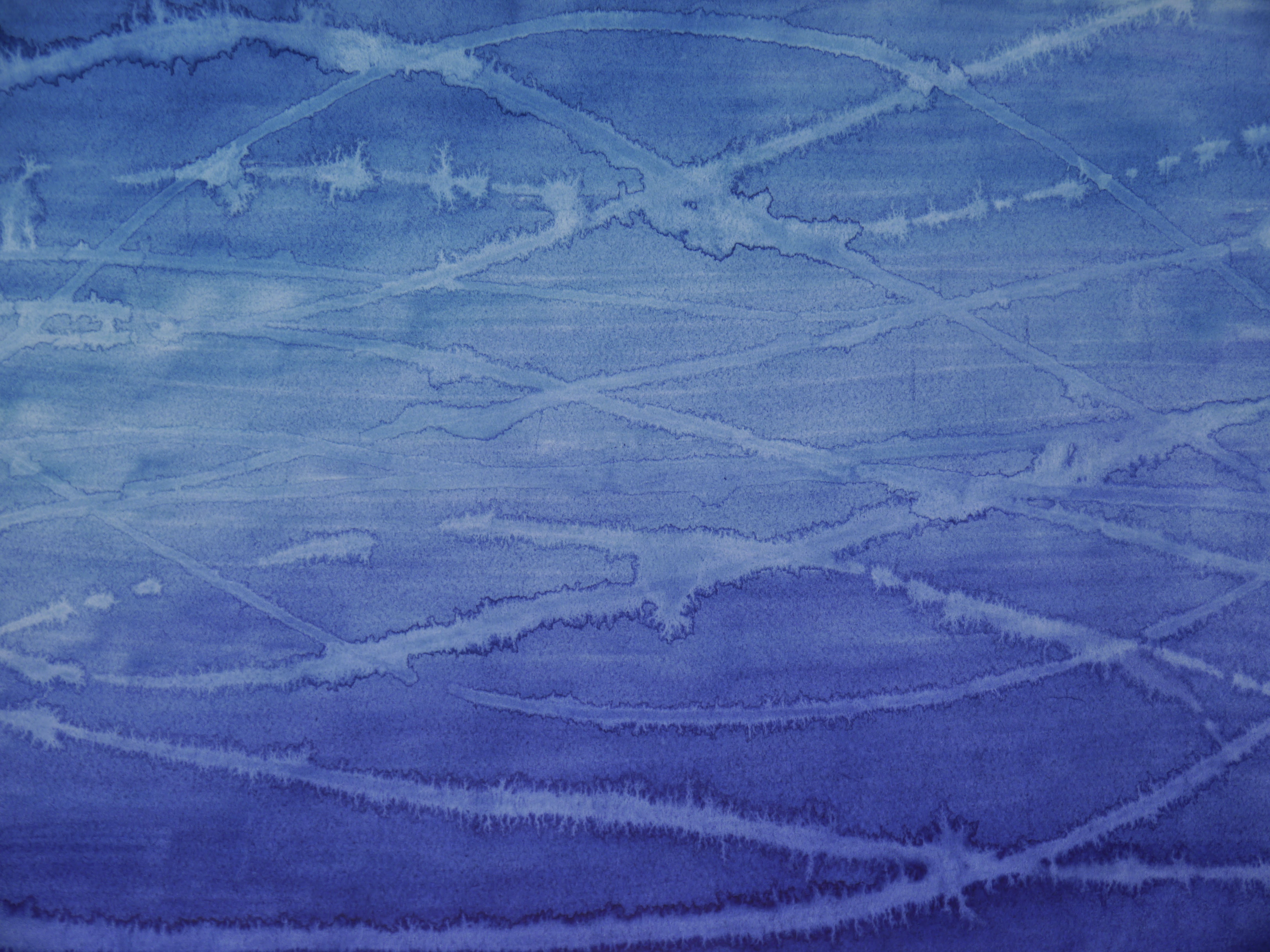
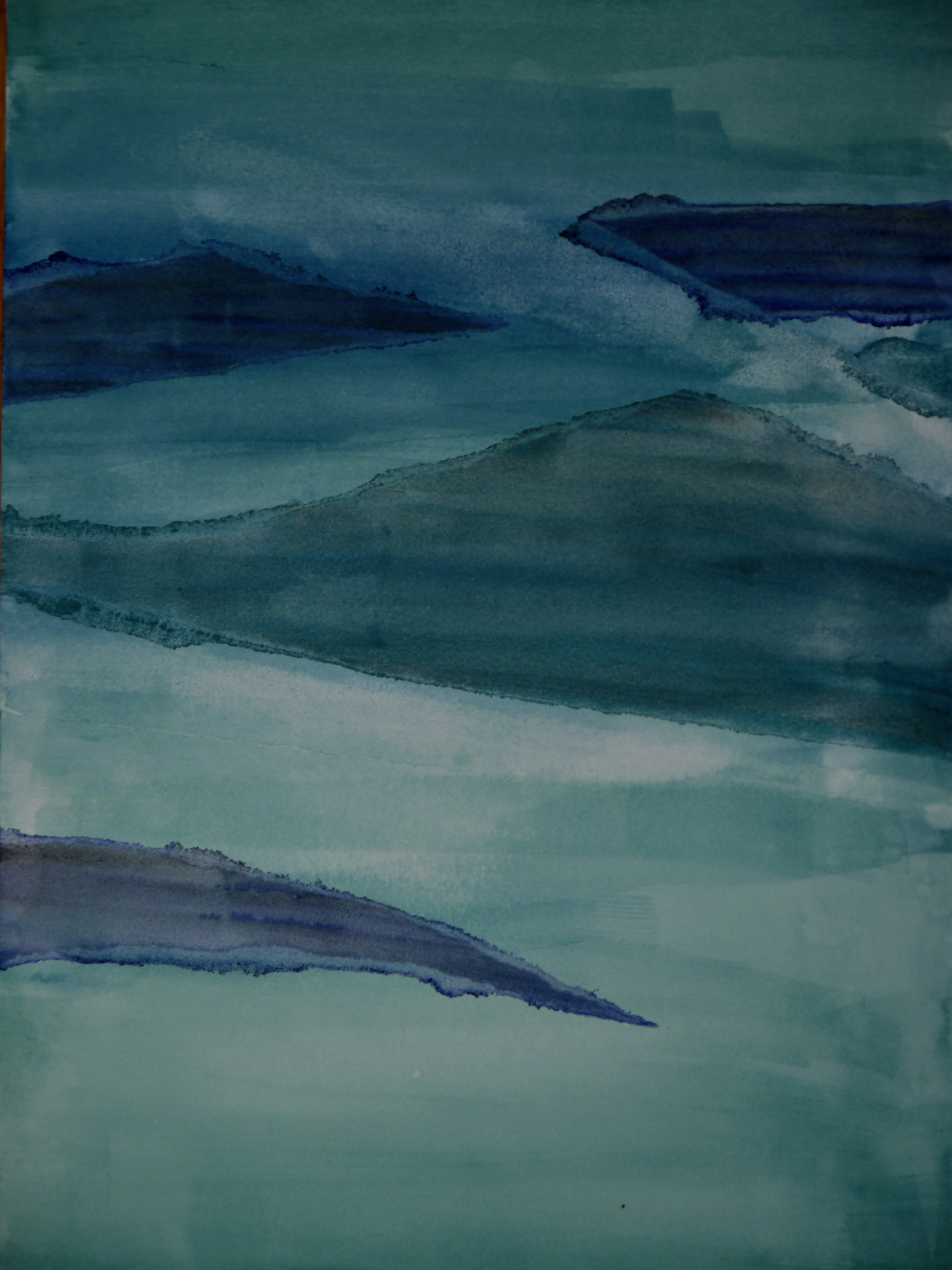
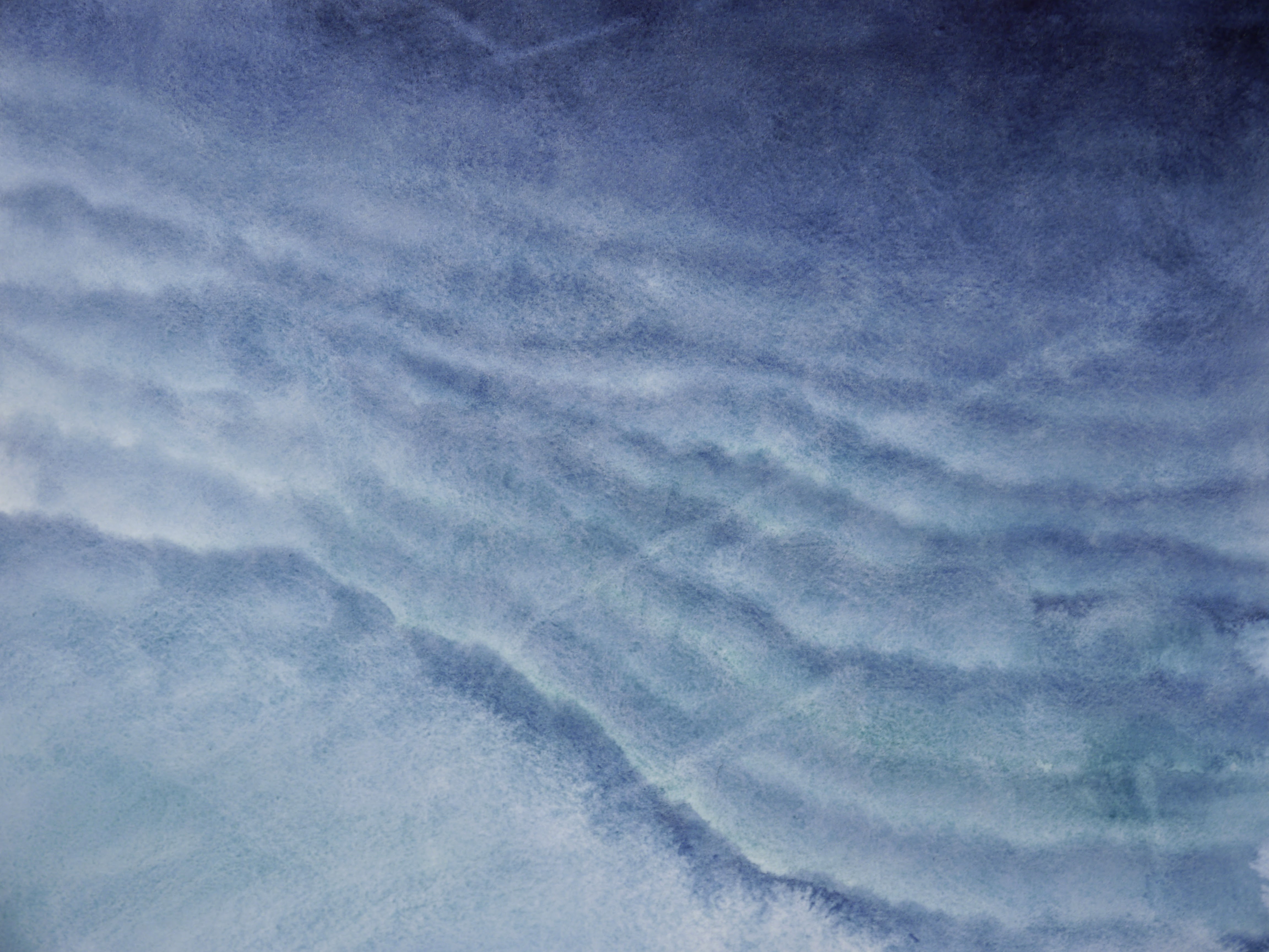
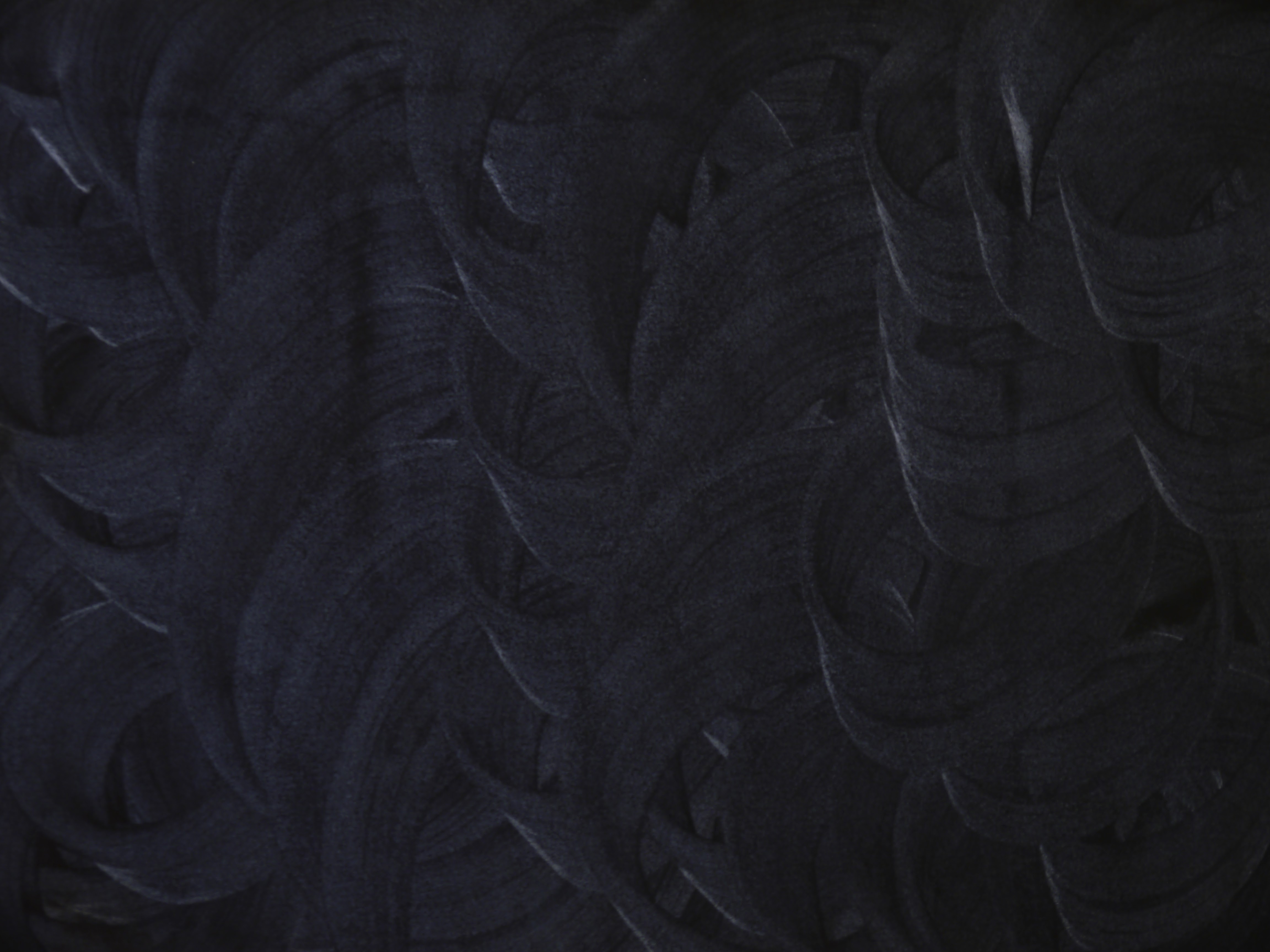
At any rate, this turned out to mostly just be a diversion: the lakeshore is already complex enough. Making consistent washes also turns out to be just as difficult as the more-gimmicky (but often beautiful!) techniques from the Internets. I also wanted to try different colors, blending between indigo and phtalo blue – but again, “simple pictures are best.” Though I did use black for the very lowest layers, it was only possible to get consistent gradients with a single hue.
-
I also mocked up the final product several times, with photos of the waterclors, shadows, etc. ↩